Data Collection

Data Collection Summary

This section provides an overview of the location of households surveyed, survey collection dates and regions, and individual survey duration.

HIT_PATH = '../../../../src/'
institution_id = 7
lang = 'en'
import os,sys, folium
sys.path.insert(0, os.path.normpath(os.path.join(os.path.abspath(''), HIT_PATH)))
import hedera_types as hedera
import odk_interface as odk

mfi = hedera.mfi(institution_id,setPathBook=True)
data = mfi.read_survey(mfi.odk_data_name)
mfi.HH = odk.households(data)

Data Collection Map

The map shows the GPS coordinates of all households covered in the mobile survey.

Note: Only the valid GPS records are shown.

import matplotlib.pyplot as plt

select = mfi.HH['GPS_Latitude']!=0
HH_with_GPS = mfi.HH[select]

# change plot layout
plt.rcParams["font.family"] = "TW Cen MT"
plt.rcParams.update({'font.size': 20})
#Define initial geolocation
lat_center = HH_with_GPS['GPS_Latitude'].mean() 
lon_center = HH_with_GPS['GPS_Longitude'].mean()
max_var = max(HH_with_GPS['GPS_Latitude'].var(),HH_with_GPS['GPS_Longitude'].var())
zoom_start = 8
if max_var>0.1:
    zoom_start -= 1
if max_var>1:
    zoom_start -= 1
initial_location = [lat_center, lon_center]

# create map
map_osm = folium.Map(initial_location, zoom_start=zoom_start)
colors = {0: hedera.tier_color(0), 1 : hedera.tier_color(1), 2 : hedera.tier_color(2), 
          3 : hedera.tier_color(3), 4 : hedera.tier_color(4), 5: hedera.tier_color(5)}
HH_with_GPS.apply(lambda row:folium.CircleMarker(location=[row["GPS_Latitude"], row["GPS_Longitude"]],
                                        radius=10,fill_color="#FF5733",popup=(row["GPS_Latitude"],row["GPS_Longitude"],row["locality"])).add_to(map_osm), axis=1)
map_osm

Survey Collection Dates

import numpy as np
S = odk.get_survey_duration(data)
dates = np.unique(np.array(mfi.HH['date']))
ind = np.arange(len(dates))
dates_plot = []
dates_labels = []

mean_e = []
mean_c = []
mean_tot = []

for d in dates:
    
    select = mfi.HH['date']== d
    dates_plot.append( sum(select) )
    dates_labels.append(d)
    
    # get surveys data on a diven date
    surveys = S[select]    
    
    selectE = surveys['electricity']>0
    surveysE = surveys[selectE]
    mean_e.append(surveysE['electricity'].mean())
    
    selectC = surveys['cooking']>0
    surveysC = surveys[selectC]
    mean_c.append(surveysC['cooking'].mean())
    
    selectT = surveys['total']>0
    surveysT = surveys[selectT]
    mean_tot.append(surveys['total'].mean())

import matplotlib.pyplot as plt

# change plot layout
plt.rcParams["font.family"] = "TW Cen MT"
plt.rcParams.update({'font.size': 20})
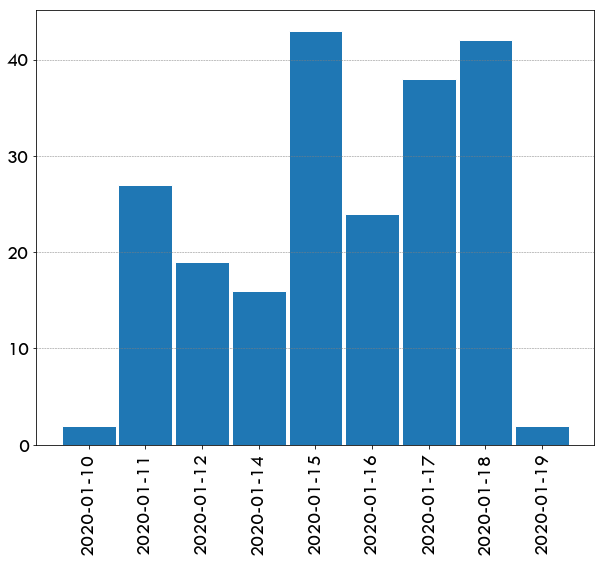
# survey per date    
fig, ax = plt.subplots(figsize=(10,8))      
plt.bar(ind, dates_plot, width=0.95,edgecolor='white')
plt.xticks(ind, dates, rotation=90)
ax.yaxis.grid(color='grey', linestyle='--', linewidth=0.5)
plt.show()

Overview of Surveys per Location

import matplotlib.pyplot as plt
plt.rcParams["font.family"] = "TW Cen MT"
plt.rcParams.update({'font.size': 14})
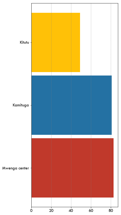
# this is needed if the surveys do not cover all states/offices
empty = []
for o in mfi.offices:
    select = mfi.HH['locality']==o
    
    if sum(select)==0:
        empty.append(o)
        
for o in empty:
    mfi.offices.remove(o)
        
mfi.plot_collection_barh()

Survey Duration

The figure shows the daily average duration of the surveys on access to electricity (Electricity) and access to modern cooking solutions (Cooking) per household.

Note: The plot only takes into account the data records with valid start and end timestamps.

import matplotlib.pyplot as plt

# change plot layout
plt.rcParams["font.family"] = "TW Cen MT"
plt.rcParams.update({'font.size': 20})
# survey duration
fig, ax = plt.subplots(figsize=(10,8))      
plt.bar(ind, mean_e, width=0.95,edgecolor='white',color='#5DADE2',label='Electricity')
plt.bar(ind, mean_c, bottom=mean_e,width=0.95,edgecolor='white',color='#DC7633',label='Cooking')
plt.xticks(ind, dates, rotation=90)
plt.legend(framealpha=1,frameon=False,bbox_to_anchor=(1.25,1.0),
                       loc='upper center').set_draggable(True)
ax.yaxis.grid(color='grey', linestyle='--', linewidth=0.85) # vertical lines
plt.show()

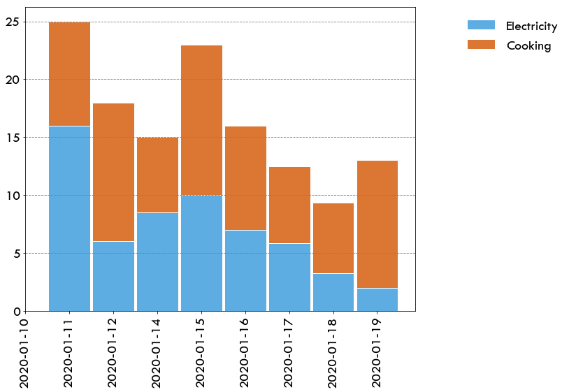
Duration of the entire interview.

Note: Some interviews only covered the household roster and are therefore much shorter.

import matplotlib.pyplot as plt

# change plot layout
plt.rcParams["font.family"] = "TW Cen MT"
plt.rcParams.update({'font.size': 20})
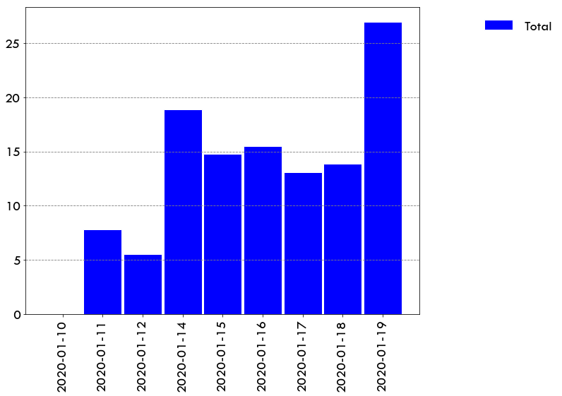
# survey duration
fig, ax = plt.subplots(figsize=(10,8))      
plt.bar(ind, mean_tot, width=0.95,edgecolor='white',color='blue',label='Total')
plt.xticks(ind, dates, rotation=90)
plt.legend(framealpha=1,frameon=False,bbox_to_anchor=(1.25,1.0),
                       loc='upper center').set_draggable(True)
ax.yaxis.grid(color='grey', linestyle='--', linewidth=0.85) # vertical lines
plt.show()

#from plotly.offline import iplot
#from plotly.offline import init_notebook_mode, plot
#from IPython.core.display import display, HTML
#import plotly as py
#import plotly.tools as tls
##print({'plotly version'+' '+py.__version__})
##py.offline.init_notebook_mode(connected=True)
#init_notebook_mode(connected=True)
##import cufflinks as cf
##cf.go_offline()
#df = data.groupby(['internal_version']).size().reset_index(name='count')
#fig = {
#    "data": [{"type": "bar",
#              "x": curps,
#              "y": surveys}],
#    "layout": {"title": {"text": "Encuestas por usuario"}}
#}
#
##df.plot(kind = 'bar', x ='internal_version', y ='count', filename = 'figure.html')
#plot(fig, filename = 'figure.html')
#display(HTML('figure.html'))